Rational Method (Q = CIA)
GIS-based estimation of the weighted runoff coefficient at the HARE diversion weir, integrating ArcMap land use, SWAT slope classes and the project's soil-group assignment. Calculations are shown with source assumptions and reproducible arithmetic.
Combined GIS analysis — infographic
This explanatory infographic is adapted from the supplied ArcMap combined-raster screenshot and the calculations used to derive the project screening coefficient; use the original GIS raster for spatial measurements. The 26 unique colors represent land-use, slope-band and soil combinations, not 26 separate land-use categories.
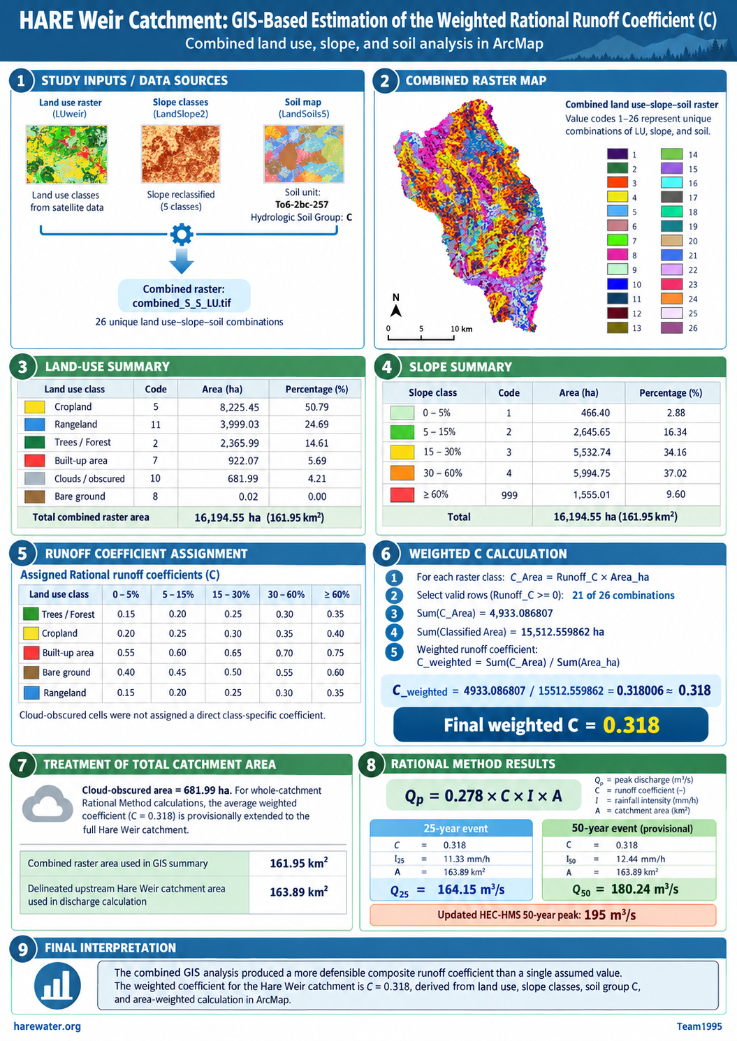
combined_S_S_LU.tif. Source: HARE GIS analysis / Team1995 · harewater.org. Note that the 50-year intensity and peak-discharge calculation are provisional.1. GIS input data and preparation
- Land cover: use the
LUweirraster with codes for trees (2), cropland (5), built-up (7), bare ground (8), cloud-obscured land (10) and rangeland (11). - Slope: derive slope bands from the DEM/SWAT
LandSlope2raster. The classes are 1 (0–5%), 2 (5–15%), 3 (15–30%), 4 (30–60%) and 999 (60% or steeper). Code 999 is a real slope class, not missing data. - Soil: use the mapped SWAT soil unit To6-2bc-257, whose
HYDGRPfield records C andTEXTURErecords LOAM. This is a project soil-group assignment, not a numerical Rational coefficient. - Combine: ArcMap Spatial Analyst → Local → Combine produced
combined_S_S_LU.tifwith 26 unique land-use–slope–soil combinations. - Raster area: output cell size 12.46159901 × 12.46159901 m. Area per cell = (X × Y) / 10,000 = 0.015529145 ha.
Three different area figures occur in the project records. The raster area is used to estimate C; the independently delineated upstream catchment is used here for Q. The earlier five-subbasin HEC-HMS model area is recorded for traceability, not silently substituted.
Land-use areas measured from the combined raster
| Land cover | Code | Area (ha) | Share (%) |
|---|---|---|---|
| Cropland | 5 | 8,225.45 | 50.79 |
| Rangeland | 11 | 3,999.03 | 24.69 |
| Trees / forest | 2 | 2,365.99 | 14.61 |
| Built-up | 7 | 922.07 | 5.69 |
| Cloud-obscured | 10 | 681.99 | 4.21 |
| Bare ground | 8 | 0.02 | 0.00 |
| Total | 16,194.55 | 100.00 | |
Slope distribution from the same raster
| Slope band | SWAT code | Area (ha) | Share (%) |
|---|---|---|---|
| 0–5% | 1 | 466.40 | 2.88 |
| 5–15% | 2 | 2,645.65 | 16.34 |
| 15–30% | 3 | 5,532.74 | 34.16 |
| 30–60% | 4 | 5,994.75 | 37.02 |
| ≥60% | 999 | 1,555.01 | 9.60 |
| Total | 16,194.55 | 100.00 | |
2. Coefficient assignment and area weighting
For the preliminary screening exercise, runoff coefficients were assigned for each mapped land-use–slope combination with the project's uniform hydrologic soil group C as context. The values below are project screening assumptions, not a table of exact coefficients prescribed by FHWA. The original mapping and slope bands remain preserved.
| Land cover | 0–5% | 5–15% | 15–30% | 30–60% | ≥60% |
|---|---|---|---|---|---|
| Trees / forest | 0.15 | 0.20 | 0.25 | 0.30 | 0.35 |
| Cropland | 0.20 | 0.25 | 0.30 | 0.35 | 0.40 |
| Built-up | 0.55 | 0.60 | 0.65 | 0.70 | 0.75 |
| Bare ground | 0.40 | 0.45 | 0.50 | 0.55 | 0.60 |
| Rangeland | 0.15 | 0.20 | 0.25 | 0.30 | 0.35 |
Verification: ArcMap Statistics for the 21 valid rows returned SUM(C_Area) = 4,933.086807 and SUM(Area_ha) = 15,512.559862, reproducing the same weighted result.
Show the full 26-combination GIS calculation table
| # | Land cover | Slope | COUNT | Area (ha) | Assigned C | C × Area |
|---|---|---|---|---|---|---|
| 1 | Cropland | 5–15% | 95,601 | 1,484.6018 | 0.25 | 371.1504 |
| 2 | Cropland | 0–5% | 15,152 | 235.2976 | 0.20 | 47.0595 |
| 3 | Cropland | 15–30% | 212,489 | 3,299.7725 | 0.30 | 989.9317 |
| 4 | Cropland | 30–60% | 180,660 | 2,805.4953 | 0.35 | 981.9234 |
| 5 | Rangeland | 15–30% | 63,560 | 987.0325 | 0.25 | 246.7581 |
| 6 | Rangeland | 5–15% | 26,756 | 415.4978 | 0.20 | 83.0996 |
| 7 | Rangeland | 0–5% | 4,073 | 63.2502 | 0.15 | 9.4875 |
| 8 | Rangeland | 30–60% | 123,185 | 1,912.9577 | 0.30 | 573.8873 |
| 9 | Trees / forest | 30–60% | 63,778 | 990.4178 | 0.30 | 297.1253 |
| 10 | Trees / forest | 15–30% | 36,908 | 573.1497 | 0.25 | 143.2874 |
| 11 | Trees / forest | 5–15% | 14,549 | 225.9335 | 0.20 | 45.1867 |
| 12 | Rangeland | ≥60% | 39,944 | 620.2962 | 0.35 | 217.1037 |
| 13 | Cropland | ≥60% | 25,776 | 400.2792 | 0.40 | 160.1117 |
| 14 | Trees / forest | 0–5% | 3,969 | 61.6352 | 0.15 | 9.2453 |
| 15 | Trees / forest | ≥60% | 33,154 | 514.8533 | 0.35 | 180.1986 |
| 16 | Cloud-obscured | 30–60% | 12,171 | 189.0052 | — | Excluded |
| 17 | Cloud-obscured | ≥60% | 1,192 | 18.5107 | — | Excluded |
| 18 | Cloud-obscured | 15–30% | 19,249 | 298.9205 | — | Excluded |
| 19 | Built-up | 5–15% | 23,507 | 365.0436 | 0.60 | 219.0262 |
| 20 | Cloud-obscured | 5–15% | 9,954 | 154.5771 | — | Excluded |
| 21 | Built-up | 15–30% | 24,074 | 373.8486 | 0.65 | 243.0016 |
| 22 | Built-up | 0–5% | 5,489 | 85.2395 | 0.55 | 46.8817 |
| 23 | Built-up | 30–60% | 6,238 | 96.8708 | 0.70 | 67.8096 |
| 24 | Cloud-obscured | 0–5% | 1,351 | 20.9799 | — | Excluded |
| 25 | Built-up | ≥60% | 69 | 1.0715 | 0.75 | 0.8036 |
| 26 | Bare ground | 15–30% | 1 | 0.0155 | 0.50 | 0.0078 |
Cloud-obscured rows are excluded from the classified-only calculation of C; their apparent C_Area = 0 is a placeholder, not an assertion of zero runoff.
3. Treatment of cloud-obscured and unrepresented land
The source image recorded 681.99 ha as cloud-obscured. Clouds are not a land-use class and were excluded when deriving C from known covers. Rather than omit that area from the screening discharge calculation, we provisionally extend the measured classified-land average C to the cloud-obscured area.
The coefficient is numerically unchanged because the missing portion was assigned exactly the calculated mean. Applying the same coefficient to the additional 194.12 ha separating the raster and the independently delineated catchment is another provisional extrapolation, not a verified land-cover measurement.
4. Rational Method peak-flow screening
The metric Rational Method relationship is Q = 0.278 × C × I × A, where discharge Q is in m³/s, C is dimensionless, intensity I is mm/h, and contributing area A is km².
The earlier time-of-concentration estimate was about 6.1 h. The reported 25-year intensity 11.33 mm/h comes from a six-hour rainfall duration, which is only an approximation to Tc. The 50-year intensity 12.44 mm/h is an unverified provisional historical input, not the updated IDF result.
Comparison with event-based modelling
| Return period | Rational Method | HEC-HMS | Interpretation |
|---|---|---|---|
| 25 years | 164.15 m³/s | 97 m³/s (earlier run) | Different input generations; not a like-for-like verification |
| 50 years | 180.24 m³/s (provisional) | ≈ 195 m³/s (updated reported peak) | Provisional Rational estimate is 7.6% lower |
5. References and related technical material
Reference formulas and selection guidance are based on the Federal Highway Administration manuals. The GIS-derived areas and numerical coefficient table are project calculations, and the class-specific C assignments should be interpreted as local screening assumptions.
- FHWA (2024a). Highway Hydrology, Hydraulic Design Series No. 2, 3rd ed. Official HDS-2 PDF ↗.
- FHWA (2024b). Urban Drainage Design Manual, Hydraulic Engineering Circular No. 22, 4th ed. Official HEC-22 PDF ↗.
- HARE Irrigation Project (2026). ArcMap
combined_S_S_LU.tif, raster attributes and SWAT soil/slope datasets. Team1995 · harewater.org.